Quantifying competition from inventory data

Where to start?

With TreeCompR, it is possible to easily compute size-distance-dependent competition indices based on inventory data. This data can be collected in the field, or derived or modeled from 3D point clouds. Depending on the input data, there are some necessary pre-processing steps. We prepared two tutorials for processing laser scanning data to obtain appropriate inventory data:

• From airborne laser scanning data to competition indices: vignette(“ALS_inventory”): ALS workflow
• From ground-based laser scanning data (from MLS/TLS) to competition indices: vignette(“TLS_inventory”): TLS workflow

Preparations

To illustrate how TreeCompR can be included inside a tidy workflow, we will make use of tidyverse functions throughout the tutorial:

library(TreeCompR)
library(tidyverse)

To highlight where they are coming from, we will explicitly quote the corresponding package for all functions used in the tutorial in the form of purrr::map() for all functions besides the magrittr pipe operator %>%.

Reading in forest inventory data with read_inv()

To be able to be parsed as a forest_inv object, inventory data must contain x and y coordinates of the individual trees (in m), and to be able to compute competition they must contain at least one size-related variable (e.g. height or diameter at breast height, or others when working with custom indices).

To ensure that the inventory data is assigned correctly, inspect the data thoroughly. Make sure to specify the units for dbh and height if they differ from the default, which is cm for dbh and m for height. Tree coordinates should always be specified in m. You can either use read_inv() to validate data.frames or paths to files with inventory data and convert them to an object type used by the TreeCompR functions, or directly pass them to compete_inv(). The former is especially useful if you have data with non-standard column names or data structures and want to have full control over how they are parsed.

Automatic column identification

In a simple case, reading data with read_inv() with standard settings (except for the metric tree diameters) looks like this:

# read inventory with diameter units set to m
inventory1 <- read_inv(
  inv_source = "data/inventory1.csv",
  dbh_unit = "m")
#> The following columns were used to create the inventory dataset:
#> id     ---     ID
#> x      ---     X
#> y      ---     Y
#> dbh    ---     DBH

If verbose = TRUE (the default), read_inv() prints the names of the main inventory variables from the original data set. This is helpful as a sanity check for the automatic column detection.

read_inv() does flexibly recognize a large number of different spellings for the common inventory variables. If provided with tabular data without explicitly specified variable names, the function by default takes the columns named “X” and “Y” (or “x” and “y”) to be the tree coordinates, and looks for columns named “height”, “height_m” or “h” as well as “dbh”, “diameter”,“diam”, or “d” (in any capitalization) as size-related variables. The tree ids are taken from columns named “id”, “tree_id”, “treeID” or “tree.id” (in any capitalization). All special characters besides “.” and “_” are stripped from the column names before matching. If verbose = TRUE, the function will inform you which columns were automatically identified to avoid errors.

The resulting “forest_inv” object looks like this (basically a modified data.table object that is printed with a header to easily identify its class).

inventory1
#> ------------------------------------
#> 'forest_inv' class inventory dataset
#> No. of obs.: 63             
#> ------------------------------------
#>             id      x      y    dbh
#>         <char>  <num>  <num>  <num>
#>  1: FASY-43-01  1.009  0.908  5.047
#>  2: ACPL-43-02 11.683  1.449  6.786
#>  3: SOAU-43-03  6.770  2.155  4.675
#> ---                                
#> 61: FASY-43-61  9.390 28.357 40.283
#> 62: FASY-43-62  5.350 27.977 32.405
#> 63: FASY-43-63 16.750 28.615 43.841

Manual column specification

If you have variable names that cannot be automatically recognized, you can specify them explicitly with the corresponding arguments either as a character string of length 1 with the variable name or by directly specifying the name without quotes. For example, assume you have a data set with (metric) UTM coordinates from a Spanish source, i.e. with “dap_cm” (diámetro en altura de pecho) instead of dbh and “altura” instead of height:

# read inventory with custom (Spanish) column titles
inventory2 <- read_inv(
  inv_source = "data/inventory2.csv",  
  x = utmx,
  y = utmy,
  dbh = dap_cm,
  height = altura,
  dbh_unit = "cm", 
  height_unit = "m")
#> The following columns were used to create the inventory dataset:
#> id     ---     automatically generated
#> x      ---     utmx
#> y      ---     utmy
#> dbh    ---     dap_cm
#> height ---     altura

Note that in this case, the function automatically generated an “id” column with ascending numbers as there was nothing in the raw data that could be automatically identified as an ID:

inventory2
#> --------------------------------------
#> 'forest_inv' class inventory dataset
#> No. of obs.: 88   No. of data cols.: 2
#> --------------------------------------
#>         id      x      y    dbh height
#>     <char>  <num>  <num>  <num>  <num>
#>  1:      1  0.573  0.168  7.232 13.168
#>  2:      2 19.330  0.844  8.064 11.565
#>  3:      3 10.182  0.383 10.779 13.615
#> ---                                   
#> 86:     86 12.829 29.278  3.713  7.780
#> 87:     87 26.712 29.375  1.641  4.306
#> 88:     88  6.962 29.644  4.585 10.219

Non-standard file formats

Non-standard field separators etc. can be internally passed on to data.table::fread() via the ... arguments to read more exotic formats such as the semicolon-separated “.csv” files with commas as decimal separators used for example in Germany. If the units are not specified explicitly, it is assumed that they are in the standard units (m for height and cm for diameter) and do not need conversion.

# read inventory with custom decimal and column separators
inventory3 <- read_inv(
  inv_source = "data/inventory3.csv", 
  dec = ",",
  sep = ";", 
  verbose = FALSE)

Additional variables

In many cases, pre-processing of the inventories based on other variables than coordinates and tree size is necessary. For that reason, it is possible to read in any objects that inherit from class data.frame (e.g., tibbles, data.tables or actual data.frames) with read_inv(). In this example, a dataset is first read in externally and filtered to get data of only one of the plots in the dataset and then read in.

# read dataset outside read_inv and filter to a single plot
dat <- readr::read_csv("data/inventory4.csv") %>% 
  dplyr::filter(plot_id == "Plot 1")
dat
#> # A tibble: 131 × 7
#>    plot_id tree_id       x        y  diam     h canopy_area
#>    <chr>     <dbl>   <dbl>    <dbl> <dbl> <dbl>       <dbl>
#>  1 Plot 1    20492 563149. 5508576. 26.0  27.4        0.755
#>  2 Plot 1    20526 563176. 5508576. 28.2  27.5        0.814
#>  3 Plot 1    20559 563144. 5508577. 50.1  33.7        0.451
#>  4 Plot 1    20563 563172. 5508576. 24.6  21.1        0.447
#>  5 Plot 1    20593 563141. 5508577. 43.4  30.1        2.04 
#>  6 Plot 1    20594 563146. 5508577. 38.9  35.5        2.56 
#>  7 Plot 1    20630 563160. 5508577. 33.2  30.3        1.22 
#>  8 Plot 1    20731 563166. 5508578.  7.28  9.15       0.680
#>  9 Plot 1    20769 563133. 5508579.  4.27  6.62       0.568
#> 10 Plot 1    20771 563145. 5508579. 42.7  31.8        0.946
#> # ℹ 121 more rows
#> # ℹ Use `print(n = ...)` to see more rows
  
# use read_inv to convert to a forest_inv object that works with TreeCompR functions
inventory4 <- read_inv(
  inv_source = dat,
  dbh = diam,
  dbh_unit = "cm", 
  height_unit = "m", 
  verbose = FALSE)
inventory4
#> ------------------------------------------
#> 'forest_inv' class inventory dataset
#> No. of obs.: 131      No. of data cols.: 2
#> ------------------------------------------
#>          id        x       y    dbh height
#>      <char>    <num>   <num>  <num>  <num>
#>   1:  20492 563148.6 5508576 25.966 27.448
#>   2:  20526 563175.9 5508576 28.151 27.527
#>   3:  20559 563144.0 5508577 50.075 33.730
#>  ---                                      
#> 129:  24253 563163.7 5508624 35.541 28.049
#> 130:  24254 563172.3 5508623 46.562 32.352
#> 131:  24255 563176.8 5508625 59.293 32.698

If there are additional columns that should be kept in the forest inventory dataset (such as the canopy area in this case), it is possible to specify keep_rest = TRUE:

# read same inventory without dropping columns
inventory4a <- read_inv(
  inv_source = dat,
  dbh = diam,
  dbh_unit = "cm", 
  height_unit = "m", 
  keep_rest = TRUE,
  verbose = FALSE)
inventory4a
#> --------------------------------------------------------------
#> 'forest_inv' class inventory dataset
#> No. of obs.: 131                          No. of data cols.: 4
#> --------------------------------------------------------------
#>          id        x       y    dbh height plot_id canopy_area
#>      <char>    <num>   <num>  <num>  <num>  <char>       <num>
#>   1:  20492 563148.6 5508576 25.966 27.448  Plot 1       0.755
#>   2:  20526 563175.9 5508576 28.151 27.527  Plot 1       0.814
#>   3:  20559 563144.0 5508577 50.075 33.730  Plot 1       0.451
#>  ---                                                          
#> 129:  24253 563163.7 5508624 35.541 28.049  Plot 1       0.602
#> 130:  24254 563172.3 5508623 46.562 32.352  Plot 1       7.765
#> 131:  24255 563176.8 5508625 59.293 32.698  Plot 1       0.634

Designating target trees with define_target()

To select target trees for computing competition indices, you can use the function define_target().

There are many different ways of specifying target trees that are described in the documentation of define_target(). Briefly, you can directly supply tree IDs as a character string, you can define them based on logical vectors, you can supply another forest_inv object created with read_tree() that contains their coordinates, or finally with a character string specifying a method to define the target trees (“buff_edge”, “exclude_edge” and “all_trees”).

Designating target trees based on subsetting

Defining targets with a vector of tree IDs could look like this, assuming you want to compute competition indices for 3 adjacent Fagus sylvatica trees and this is your naming scheme:

# set target trees based on character vector with tree ids
targets1 <- define_target(
  inv = inventory1, 
  target_source = c("FASY-43-24", "FASY-43-27", "FASY-43-30")
)
targets1
#> ----------------------------------------------------
#> 'target_inv' class inventory with target definitions
#> No. of obs.: 63                 No. of data cols.: 1
#> No. of target trees: 3       Target source: tree IDs
#> ----------------------------------------------------
#>             id      x      y target    dbh
#>         <char>  <num>  <num> <lgcl>  <num>
#>  1: FASY-43-01  1.009  0.908  FALSE  5.047
#>  2: ACPL-43-02 11.683  1.449  FALSE  6.786
#>  3: SOAU-43-03  6.770  2.155  FALSE  4.675
#> ---                                       
#> 61: FASY-43-61  9.390 28.357  FALSE 40.283
#> 62: FASY-43-62  5.350 27.977  FALSE 32.405
#> 63: FASY-43-63 16.750 28.615  FALSE 43.841

Objects of class “target_inv” are “forest_inv” type forest inventory datasets that have an additional target column with a logical “target” vector that identifies the target trees.

To visually inspect the position of the designated target trees relative to the other trees in the neighborhood, you can use the function plot_target(), which automatically displays the relevant information depending on the target_source setting for both target_inv datasets and the output of compete_inv() itself. Here is a plot of the target trees with a buffer of 10 m which is fully surrounded by other trees, showing that it is possible to calculate competition indices with a 10 m search radius for the three targets:

plot_target(targets1, radius = 10)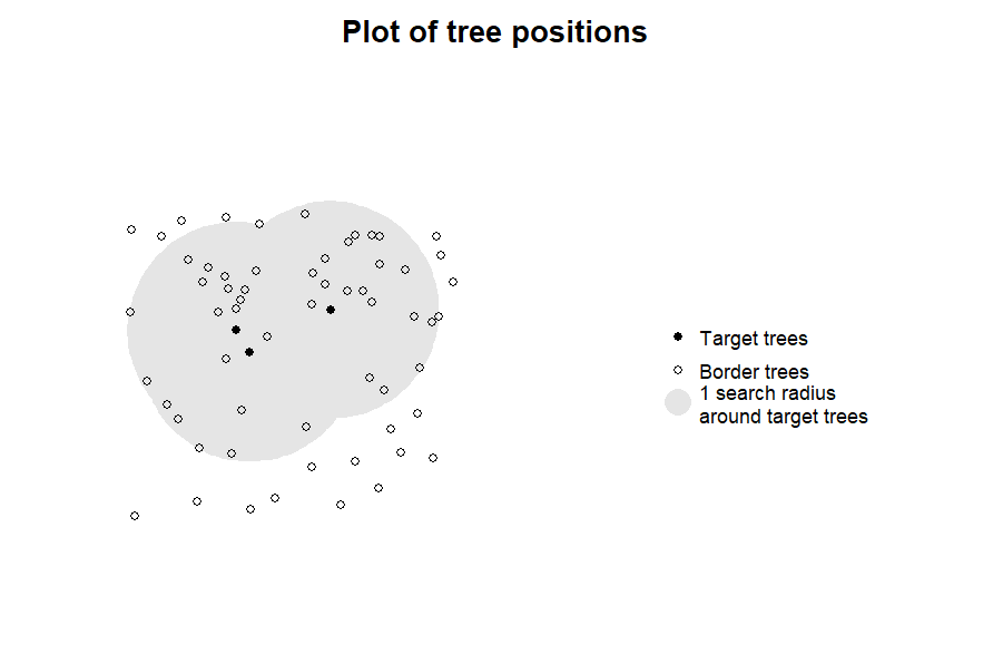

The purpose of this function is to provide a fast tool for visual inspection rather than to create beautiful visual output. As all the data for the plot are contained in the target_inv object, more appealing (e.g., ggplot2-based) visualizations are left as an exercise to the user.

You might also want to define target trees based on a logical criterion, for instance for all trees whose ID contains “FASY”:

# set target trees based on logical vector
targets2 <- define_target(
  inv = inventory1, 
  target_source = grepl("FASY", inventory1$id)
  )
# visual inspection
plot_target(targets2, radius = 10)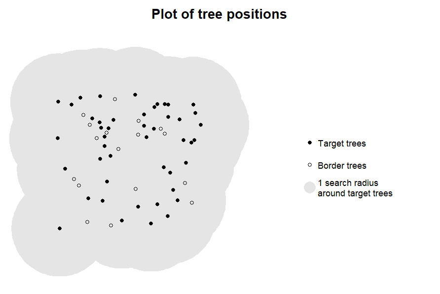

In this case, the plot of the target trees shows that many of the target trees are situated on the plot border, which would result in edge effects. In such cases, we strongly advice against computing indices for these trees (see below). To avoid calculating competition indices in situations where it is not appropriate, we recommend to make plotting with plot_target() a standard step of your workflow.

Designating target trees based on coordinates from other data sources

In many cases you will have target tree coordinates that come from a different data source and have a different accuracy than the inventory data, for instance when you perform a ground-based study focusing on single trees and wish to derive tree competition from ALS sources based on the GPS coordinates from your trees. In these cases, you will have to match the GPS coordinates against the tree coordinates derived from the ALS source (see ALS workflow for details on how to derive inventory data from ALS sources).

In these cases, it is possible to supply an inventory based on a second set of coordinates as a target_source which is then matched against the inventory data. IDs are then ignored (as they are likely automatically generated anyway) and matching is based only on the closest trees within a buffer of tol m (the default is tol = 1: matching within 1 m). All further size-related variables in the second set of coordinates are ignored as well to ensure the competition indices are based on the same data source. Here, GPS coordinates for 15 trees are read in and matched against the data in the inventory.

# designate target trees based on GPS coordinates
# read target tree positions
(target_pos <- read_inv(
  "data/target_tree_gps.csv", x = gps_x, y = gps_y))
#> ------------------------------------
#> 'forest_inv' class inventory dataset
#> No. of obs.: 15                     
#> ------------------------------------
#>          id        x       y
#>      <char>    <num>   <num>
#>  1: FASY-01 563157.6 5508615
#>  2: FASY-02 563141.8 5508602
#>  3: FASY-03 563147.0 5508610
#> ---                         
#> 13: FASY-13 563161.4 5508611
#> 14: FASY-14 563154.7 5508609
#> 15: FASY-15 563140.0 5508607

# define target trees
targets3 <- define_target(
  inv = inventory1, 
  target_source = target_pos,
  tol = 1 # match within 1 m accuracy
  )
# visual inspection
plot_target(targets3, radius = 8)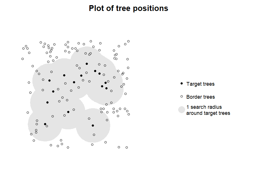

For the intended 8 m search radius, these coordinates are appropriate.

If no trees in the inventory are within the desired tolerance of one or more of your target trees, or if several target trees are in within the tolerance, you will receive a warning. If there is more than one tree that is an equally good match for a target tree within 5 cm difference, the function will fail with an error.

In cases where you have additional data sources that can be used for matching (e.g. if you know the height of the trees from the field and can use this as an additional information source) or when high tree densities and low GPS accuracy make automated matching difficult, it may be advisable to do the matching outside TreeCompR and define the target trees by ID or logical subsetting instead.

Designating target trees based on spatial arrangement

In many cases, there will be no list of a priori specified target trees, and the aim will be to calculate valid competition indices for as many trees as possible. In these cases, we recommend to use target_source = "buff_edge". This automatically designates all trees in the plot that are at least one search radius away from the plot edge (roughly approximated by a concave hull) to avoid edge effects. This is particularly important for TLS/MLS data and traditional forest inventories, which, unlike ALS-derived datasets, tend to cover relatively small forest plots rather than entire forests. Setting target_source = "exclude_edge" only removes the trees on the edge of the plot without checking how close the rest of the trees is from the edge and is hence less restrictive but more prone to edge effects than the previous option. If you use these spatially explicit methods of defining target trees, make sure that your inventory only contains data from one plot as currently grouping is not possible in define_target(). If you want to consider doing this for a larger number of plots, consider e.g. mapping over the plots with [purrr::map()] to compute the output step by step.

Here is an example of how to identify all potential target trees that run in no risk of excluding potential edge trees when computing competition indices for the same tree as in the previous example, again with a search radius of 8 m:

# designate target trees with a 10 m buffer to the plot border
targets4 <- define_target(
  inv = inventory4, 
  target_source = "buff_edge", 
  radius = 8)
# visual inspection
plot_target(targets4)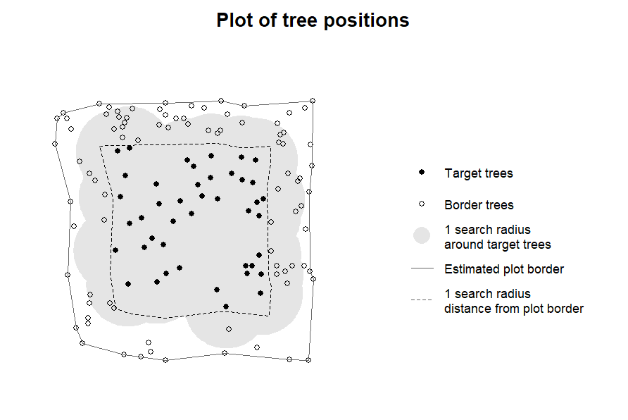

In this case, the radius does not have to be specified in plot_target() as the radius used for the buffer is stored in the attributes of the “target_inv” object.

Doing the same with target_source = "exclude_edge" results in the following:

# designate target trees by only excluding the plot border
targets5 <- define_target(
  inv = inventory4, 
  target_source = "exclude_edge",
  radius = 8)
# visual inspection
plot_target(targets5)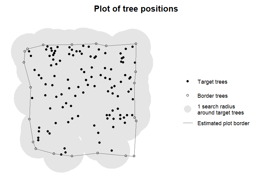

It can be seen that only the trees that are directly on the plot border were removed. The radius in this case is again passed on to plot_target(), but in this case only used to determine the minimum possible distance between two edge trees for the concave hull algorithm. This method of determining edge trees is considerably less restrictive than “buff_edge”, and in this case resulted in a large number of trees with buffers extending further than the plot. We therefore recommend to be careful with this setting.

If a certain amount of overlap between the plot border and buffers of individual trees is permitted it is usually better to use “buff_edge” with a radius below the intended search radius as it maintains a constant distance.

Designating all trees as target trees

While it is possible to compute competition indices for all trees (target_source = "all_trees"), this results in a warning and should only be done if there are very good reasons to assume that the edge trees in the data are actually situated at the forest edge, as otherwise there will be intense edge effects: for a tree on a straight plot edge, on average nearly half and for a tree in an edge position in a rectangular plot 3/4 of the competitors will be missing in the data! Therefore, this setting should only be used for ALS derived data where it is clear that a whole forest is being used as input.

# designate all trees as target trees
targets6 <- define_target(
  inv = inventory4, 
  target_source = "all_trees")
#> Warning message:
#> In define_target(inv = inventory4, target_source = "all_trees") :
#>   Defining all trees as target trees is rarely a good idea. Unless your
#> forest inventory contains all trees in the forest, this will lead to strong
#> edge effects. Please make sure that this is really what you want to do.

# visual inspection
plot_target(targets6, radius = 8)
#> Warning message:
#> In plot_target(targets6, radius = 8) :
#>   All trees in the dataset are defined as as target trees.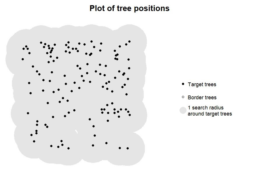

Computing competition indices with compete_inv()

Basic usage

compete_inv() is very flexible with its input, in essence directly accepting everything that can also be loaded with read_inv() and also passing additional settings for column specifications etc. on to this function, which is then used to load the data internally. In addition, all options for target_source that can be set in define_target() can be directly specified in compete_inv(). In consequence, in most use cases this function will likely be called directly unless there are reasons to perform the other steps explicitly, for instance, because the data structure and formatting differ between the inventory and target files and require different sets of custom column name settings, or because an inspection of the target settings and spatial configuration is desired before computing the results (which is certainly a good idea for large datasets).

To identify the neighbor trees within the search radius of each target tree, compete_inv()uses the function knn() from package nabor that is based on a very efficient C++ implementation of the k-nearest neighbor algorithm from libnabo. This makes it possible to deal with very large inventory datasets in a relatively fast way as the pairwise distances of far-away trees are never actually evaluated. In order to do this, it is necessary to specify a maximum number of nearest neighbors to consider for each tree, which has to be sufficiently larger than the maximum number of trees expected in a search radius (kmax, by default 999). The function then identifies which among the nearest neighbors are within the search radius.

For most datasets, the choice of kmax will not play a role as search radii large enough to contain that many trees rarely make sense from a biological perspective, and because in many cases performance differences between different values of kmax will hardly be notable. However, for very large inventory datasets, as can be expected when working with ALS data sources, The performance difference compared to the regular pairwise-distance-based implementations as e.g. sf::st_is_within_distance() can be several orders of magnitude. As a practical example, evaluating sf::st_is_within_distance() with a search radius of 10 m for 38,522 trees from an ALS inventory on a modern laptop took 750.73 sec (around 12 min 31 sec), while computing the Braathe index with the same settings for all these trees withcompete_inv() took 16.38 seconds.

In our performance tests, using compete_inv() with the built-in indices and standard settings was reasonably fast for datasets with up to several tens of thousands of trees, with computation times mostly below a minute. For larger inventories, it may be beneficial to use parallel computing, which in our package is implemented via the foreach package and the doParallel backend (see below for more details).

If target trees have already been specified with target_inv(), the outcome can directly be passed to compete_inv(), which then ignores the target_source argument and all further arguments that are passed on to read_inv() and define_target().

# compute Hegyi index based on existing 'target_inv' object
 (CI1 <- compete_inv(inv_source = targets4, radius = 8, 
                    method = "CI_Hegyi"))
#> ------------------------------------------------------------
#> 'compete_inv' class distance-based competition index dataset
#> No. of target trees: 43     Source inventory size: 131 trees
#> Target source: 'buff_edge' (8 m)          Search radius: 8 m
#> ------------------------------------------------------------
#>         id        x       y    dbh height CI_Hegyi
#>     <char>    <num>   <num>  <num>  <num>    <num>
#>  1:  21277 563160.3 5508586  9.863 12.098    0.952
#>  2:  21512 563166.9 5508589 11.917 12.720    4.971
#>  3:  21581 563158.5 5508589 12.085 14.659    0.937
#> ---                                               
#> 41:  23501 563157.4 5508615 26.787 27.172    2.286
#> 42:  23582 563139.6 5508616  9.186 11.461    6.138
#> 43:  23652 563141.8 5508616 11.017 13.886    5.866

The resulting “compete_inv” object contains only the target trees, and has one additional column for each computed competition index. Information about the neighbor trees as well as information about the methods are stored as attributes.

In addition to analyses based on existing “target_inv” objects, it is possible to read data from file, for example from a “.csv” source with non-standard column names and decimal and field separators (in this example, from a German file source):

CI2 <- compete_inv(
  inv_source = "data/inventory5.csv",
  target_source = "buff_edge",
  radius = 10, 
  method = "CI_Hegyi",
  x = Koord_x, 
  y = Koord_y,
  id = Baumname,
  dbh = Durchmesser,
  sep = ";",
  dec = ","
  )
#> The following columns were used to create the inventory dataset:
#> id     ---     Baumname
#> x      ---     Koord_x
#> y      ---     Koord_y
#> dbh  ---   Durchmesser

The output of this function can then again be inspected in the same way as above using plot_target() to make sure the selection of target trees make sense:

plot_target(CI2)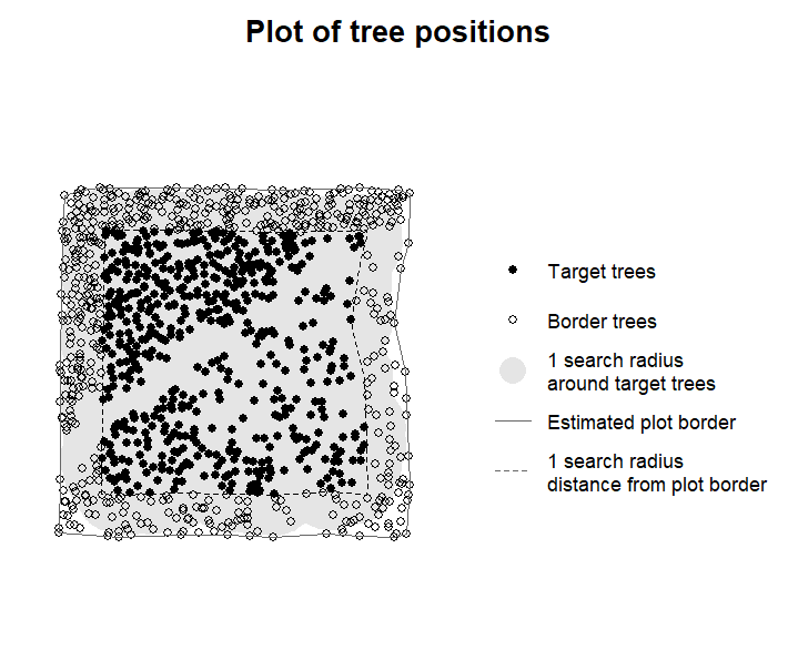

Available competition indices

The function computes a series of inventory-based competition indices commonly used in the literature that can be specified via the method argument (Hegyi 1974; Braathe, 1980; Rouvinen & Kuuluvainen, 1997; see also Contreras et al., 2011). These are either based on tree diameter at breast height (“CI_Hegyi”, “CI_RK1”, “CI_RK2”) or on tree height (“CI_Braathe”, “CI_RK3”, “CI_RK4”).

The competition indices are computed according to the following equations, where $d_i$ and $h_i$ are the dbh and height of neighbor tree $i$, $d$ and $h$ are dbh and height of the target tree, and $dist_i$ is the distance from neighbor tree $i$ to the target tree.

Diameter-based competition indices

CI_Hegyi introduced by Hegyi (1974): $$CI_{Hegyi} = \sum_{i=1}^{n} \frac{d_{i}} {d \cdot dist_{i}}$$CI_RK1 according to CI1 Rouvinen & Kuuluvainen (1997): $$CI_{RK1} = \sum_{i=1}^{n} \mathrm{arctan}\left(\frac{d_{i} } {dist_{i}}\right)$$CI_RK2 according to CI3 in Rouvinen & Kuuluvainen (1997): $$CI_{RK2} =\sum_{i=1}^{n} \frac{d_{i}}{d} \cdot \mathrm{arctan}\left(\frac{d_{i} } {dist_{i}}\right)$$

Height-based competition indices

CI_Braathe according to Braathe (1980): $$CI_{Braathe} = \sum_{i=1}^{n} \frac{h_{i}}{h \cdot dist_{i}}$$CI_RK3 according to CI5 in Rouvinen & Kuuluvainen (1997): $$CI_{RK3} = \sum_{i=1}^{n} \mathrm{arctan}\left(\frac{h_{i}}{ dist_{i}}\right)$$ for all trees with $$h_{i} > h$$CI_RK4 based on CI3 in Rouvinen & Kuuluvainen (1997) and Contreras et al. (2011): $$CI_{RK4} = \sum_{i=1}^{n} \frac{h_{i}}{ h } \cdot \mathrm{arctan}\left(\frac{h_{i}}{ dist_{i}}\right)$$

Generic size-based Hegyi-type competition index

CI_size based on Hegyi (1974), but with a user-specified size-related variable ($s_i$: size for neighbor tree $i$, $s$: size of the target tree): $$CI_{size} = \sum_{i=1}^{n} \frac{s_{i}}{s \cdot dist_{i}}$$

An advantage of the classical distance-based indices (CI_Hegyi and CI_Braathe) is their clear interpretation as the sum of the relative sizes of the neighbor trees relative to the target tree size, weighted by their distance to the target tree.

If method = "all_methods" (the standard setting), compete_inv() computes all indices that can be computed with the data available in the inventory.

CI3 <- compete_inv(inv_source = targets4, 
                    radius = 8, method = "all_methods")
CI3[, -c(2:3)] # remove coordinates to make room for printing
#> ------------------------------------------------------------------------
#> 'compete_inv' class distance-based competition index dataset
#> No. of target trees: 43                 Source inventory size: 131 trees
#> Target source: 'buff_edge' (8 m)                      Search radius: 8 m
#> ------------------------------------------------------------------------
#>         id    dbh height CI_Hegyi CI_RK1 CI_RK2 CI_Braathe CI_RK3 CI_RK4
#>     <char>  <num>  <num>    <num>  <num>  <num>      <num>  <num>  <num>
#>  1:  21277  9.863 12.098    0.952  4.233  6.599      0.909  3.702  6.208
#>  2:  21512 11.917 12.720    4.971 14.872 38.159      4.098 13.663 30.618
#>  3:  21581 12.085 14.659    0.937  4.258  7.277      0.843  2.663  6.439
#> ---                                                                     
#> 41:  23501 26.787 27.172    2.286 15.139 17.242      1.849  8.308 13.240
#> 42:  23582  9.186 11.461    6.138 16.847 43.552      4.679 14.254 32.146
#> 43:  23652 11.017 13.886    5.866 17.400 42.582      4.354 12.267 30.132

In this example, the inventory contained both dbh and height, but no user-specified size, and accordingly all built-in indices except the CI_size are included in the output.

Choosing a search radius

All indices that can be calculated with compete_inv() are based on a distance-weighted sum of the relative size of all neighbor trees within the search radius compared to the size of the central tree, or a sum of a transformation thereof. As the search radius determines how many trees are included for calculating these metric for each tree, all these distance-based competition indices are extremely sensitive to the choice of the search radius. An obvious consequence of this is that it is not possible to meaningfully compare distance-based competition indices calculated with different search radii. Perhaps less obvious is that the optimal search radius may differ between species, as different tree species have different average sizes and rooting patterns, and that comparisons between species using competition indices calculated with the same settings may not always yield meaningful results. Some authors recommend using a search radius based on the average crown size of the trees in the plot, such as Lorimer (1983), who suggests a search radius of 3.5 average crown radii. While such a recommendation certainly makes more sense than sticking to standard values such as 10 m, regardless of whether you are calculating competition for stunted Elfin forests or gigantic Redwood trees, ultimately such a setting will always be arbitrary and there are limits to the comparability of indices between studies and between species.

User-specified competition indices

With TreeCompR, defining user-specified competition indices is very easy. All it takes is to write a function that takes the arguments target and neigh as its inputs, and returns a single numeric value (the value of the competition index for the current tree) as an output. Here target is a single-line “forest_inv”-based data.table with the data of a target tree, and neigh is a multi-line “forest_inv”-based data.table with the data of all neighbor trees of the target tree (including their distance “dist` to the target tree). This function will then be evaluated for all target trees to calculate their value of the index.

For instance, a working version of the Hegyi index can be defined like this:

CI_Hegyi_new <- function(target, neigh)  sum(neigh$dbh / (target$dbh * neigh$dist))

This function can then be called with the method argument compete_inv() as a competition index:

compete_inv(inv_source = targets4, radius = 8,
            method = c("CI_Hegyi", "CI_Hegyi_new"))
#> ---------------------------------------------------------------
#> 'compete_inv' class distance-based competition index dataset
#> No. of target trees: 43        Source inventory size: 131 trees
#> Target source: 'buff_edge' (8 m)             Search radius: 8 m
#> ---------------------------------------------------------------
#>         id        x       y    dbh height CI_Hegyi CI_Hegyi_new
#>     <char>    <num>   <num>  <num>  <num>    <num>        <num>
#>  1:  21277 563160.3 5508586  9.863 12.098    0.952        0.952
#>  2:  21512 563166.9 5508589 11.917 12.720    4.971        4.971
#>  3:  21581 563158.5 5508589 12.085 14.659    0.937        0.937
#> ---                                                            
#> 41:  23501 563157.4 5508615 26.787 27.172    2.286        2.286
#> 42:  23582 563139.6 5508616  9.186 11.461    6.138        6.138
#> 43:  23652 563141.8 5508616 11.017 13.886    5.866        5.866

The output is identical to the built-in function.

This feature can also be used to modify existing indices, e.g. by calculating the RK2 index only for trees that are taller than the target tree:

CI_RK1_tall <- function(target, neigh) 
  CI_RK1(target, neigh[neigh$height > target$height, ])

In many cases, it can e.g. be interesting to split up the contribution to the total competition by different competitor species (see Hajek et al., 2022 for an example). This can be done analogously, for example for a mixed stand of hornbeam, oak and ash:

# define partial index for oak
CI_Hegyi_QURO <- function(target, neigh) 
  CI_Hegyi(target, neigh[neigh$species == "Quercus robur", ])
# define partial index for hornbeam
CI_Hegyi_CABE <- function(target, neigh) 
  CI_Hegyi(target, neigh[neigh$species == "Carpinus betulus", ])
# define partial index for ash
CI_Hegyi_FREC <- function(target, neigh) 
  CI_Hegyi(target, neigh[neigh$species == "Fraxinus excelsior", ])

# load complete dataset (keep rest: information about species etc is maintained)
inv_species <- read_inv("data/inventory6.csv", keep_rest = TRUE)
form(inv_species)
#> -----------------------------------------------------------
#> 'forest_inv' class inventory dataset
#> No. of obs.: 597                       No. of data cols.: 3
#> -----------------------------------------------------------
#>          id      x       y    dbh height            species
#>      <char>  <num>   <num>  <num>  <num>             <char>
#>   1:  22059  7.077   0.187 39.001 31.559      Quercus robur
#>   2:  22061 18.967   0.518 42.586 32.799 Fraxinus excelsior
#>   3:  22062 27.169   0.647  3.440  6.623      Quercus robur
#>  ---                                                       
#> 595:  29263  8.327  98.759 41.372 36.088      Quercus robur
#> 596:  29388 47.928 100.059 57.913 33.186      Quercus robur
#> 597:  29429 35.799 100.089 37.972 29.876      Quercus robur


# compute species-decomposed Hegyi
comp_species <- compete_inv(
  inv_source = inv_species, target_source = "buff_edge", radius = 12, 
  method = c("CI_Hegyi_QURO", "CI_Hegyi_CABE", "CI_Hegyi_FREC", "CI_Hegyi"))
> comp_species[, c(1, 6:9)] # only show ID and indices
#> --------------------------------------------------------------
#> 'compete_inv' class distance-based competition index dataset
#> No. of target trees: 350      Source inventory size: 597 trees
#> Target source: 'buff_edge' (12 m)          Search radius: 12 m
#> --------------------------------------------------------------
#>          id CI_Hegyi_QURO CI_Hegyi_CABE CI_Hegyi_FREC CI_Hegyi
#>      <char>         <num>         <num>         <num>    <num>
#>   1:  23028         2.604         1.164         1.005    4.773
#>   2:  23029         2.685         1.805         1.659    6.149
#>   3:  23030         3.319         1.213         1.961    6.493
#>  ---                                                          
#> 348:  28457         1.947         0.601         0.431    2.979
#> 349:  28485         4.910         5.807         1.817   12.534
#> 350:  28534         8.705         6.316         0.904   15.925

As in the plot the three species are the only species that occur, this constitutes a full decomposition of the Hegyi index into the contributions of different competitor species:

# test if the decomposition worked
with(comp_species, 
     all.equal(CI_Hegyi_QURO + CI_Hegyi_CABE + CI_Hegyi_FREC, CI_Hegyi))
#> [1] TRUE

As species-specific directed interaction are likely very common among competing tree species, such a decomposition may often be more beneficial for understanding competition between trees than looking at the overall effect of competition.

Parallel computing with compete_inv()

if you have inventory datasets with substantially more than 100000 trees, as is possible when using ALS sources, the computation time for the indices in compete_inv() may become limiting. In such cases, the computation can be performed in parallel using parallelize = TRUE. In this case, the function internally registers a cluster using doParallel::registerDoParallel() with a number of cores specified via the cores argument. doParallel acts as a backend for foreach::foreach() and uses the parallel package to split the computations for the loop for the competition indices on several cores.

The standard for cores is to take the value registered in options("cores")[[1]]. If this value is NULL, by default it uses ⁠parallel::detectCores() to detect the number of cores.

An example running compete_inv() on 8 processor cores for a large dataset is provided here:

large_inv <- compete_inv(
  inv_source = "data/very_large_inv.csv", 
  target_source = "buff_edge", 
  method = "CI_Hegyi",
  radius = 12,
  kmax = 100,           # a minor speedup is possible by using lower values for kmax
  parallelize = TRUE,   # use parallel computing...
  cores = 8             # ...on 8 processor cores
)

As setting up and registering the cluster can take a certain time, our benchmarks indicate that the speedup by running the computation on multiple cores does not really pay off for datasets below 100000 trees, but when the numbers go in the millions it can strongly speed things up, though above a certain point it is most likely better to split the analysis into chunks that are analyzed separately.