Quantifying competition from point cloud data

Getting started

Before you can start computing competition indices based on point cloud data from terrestrial or mobile laserscanning with TreeCompR, these data have to be thoroughly vetted and pre-processed. In this tutorial, we will first summarize our main recommendations for the handling and preprocessing of point-cloud data, and then explain how to use compete_pc() and the associated TreeCompR functions to compute competition indices.

To illustrate how TreeCompR can be included inside a tidy workflow, we will make use of tidyverse functions throughout the tutorial:

library(TreeCompR)
library(tidyverse)

To highlight where they are coming from, we will explicitly quote the corresponding package for all functions used in the tutorial in the form of purrr::map() for all functions besides the magrittr pipe operator %>%.

Pre-processing the point clouds

Before using the cone and cylinder point cloud approaches, the trees for which competition is to be quantified must be extracted from the plot. The most accurate (if time consuming) way to do this is by manual segmentation, for instance with CloudCompare. Make sure that the point cloud is ready to use (e.g. co-registration of the TLS scans, or any filtering of outliers should be done beforehand).

In CloudCompare, load your point cloud of the whole plot and use the Segment function to extract the target tree. Make sure you do not miss any part or include neighboring trees or their branches, as it is crucial to determine which parts of the point cloud belong to neighbors and which points belong to the target tree. Pay particular attention to the ground and do not include any ground points in your target tree’s point cloud, otherwise the tree’s base position may be determined imprecisely in later steps as the tree_pos() function is based on the lowest points in the point cloud of the target tree.

Methods Workflow

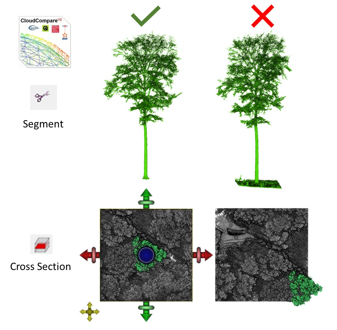
After extracting the target tree, export the point cloud by selecting the file in the DB Tree and click File - Save. Do the same for the whole plot, but first clip the point cloud to your area of interest. The best way to do this is to select top view and use the Cross Section function to clip your point cloud. Make sure that your target tree is not at the edge of the plot. For the example dataset in our paper, we used 30 x 30 m plots.

When exporting/saving the point clouds, you can select .las/.laz, .txt, .csv, … TreeCompR is flexible with file formats, but if possible, use the same format for target trees and their neighborhoods, as there may be slight numeric differences between formats that complicate coordinate matching.

After clicking save, you will be asked to select the output resolution. If you choose a custom resolution or coordinate accuracy, make sure you choose the same for the target tree and the neighborhood cloud! In our examples, we rounded our coordinates to 2 decimal places (i.e. to 1 cm accuracy), which also is what the compete_pc() uses by default for coordinate matching, but other values are possible.

Quantifying competition with TreeCompR

Once you have the two point clouds for target tree and neighborhood, you can use the read_pc() function of TreeCompR to read and validate them, or directly pass the paths to the point clouds to compete_pc(). Methods Workflow

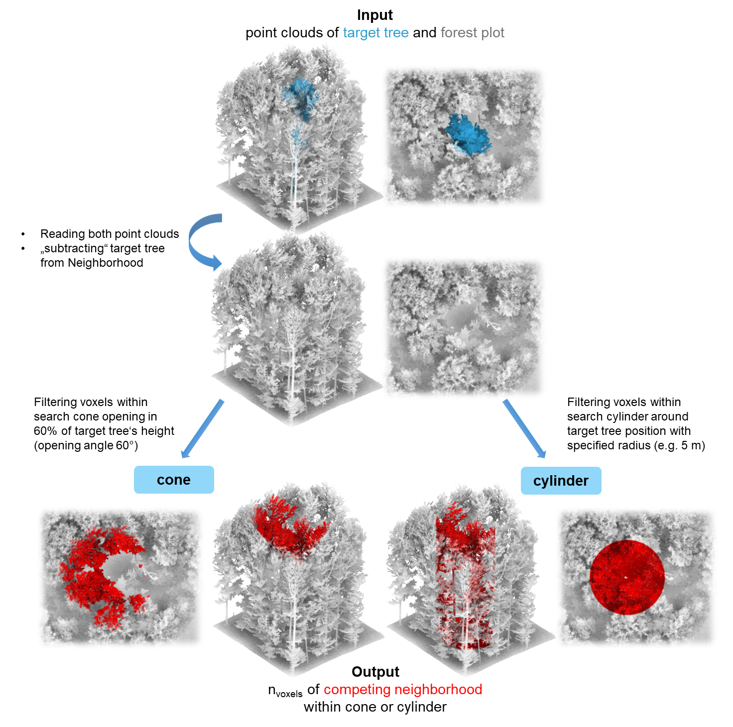
Basic use of `compete_pc()`

In compete_pc(), you can select the method for computing competition indices by setting comp_method to "cylinder", "cone" or "both". To compute the competition indices for either of these methods, the position of the center of the cone or cylinder has to be defined. The center_position argument allows to center the cone or cylinder either around the central point of the crown projected area ("crown_pos") or the central point of the tree base ("base_pos"). Usually, the position of a tree is calculated by using the lowest points of a tree and take the mean or median. However, if a tree is not growing straight and we want to identify (crown-)competition, we think it is more reasonable to instead focus on the center of the crown. For that reason, compete_pc() currently defaults to center_position = "crown_pos", the median of the x and y position of the voxelized crown projected area (see the documentation of tree_pos() for details).

If you want to use the stem base position, there are additional parameters that you can adjust to ensure the correct position determination, namely h_xy (range in m above the lowermost point of the tree point cloud the base position should be calculated from) and z_min (minimum number of points in the lowermost layer of voxels used to calculate base position of the tree). More about the methods themselves and the settings and sensitivity can be found in Seidel et al. (2015), Metz et al. (2013), or, for the original KKL index, in Pretzsch et al. (2002).

In the following example, the compete_pc is used to calculate both cone and cylinder-based competition indices centered around the crown center, with a cone opening in a height of 0.6 times the total target tree height and a cylinder radius of 4 m:

# compute competition indices
CI1 <- compete_pc(
forest_source = "data/neighborhood.txt", 
tree_source   = "data/tree.txt", 
comp_method   = "both",        # calculate CI in cylinder and cone
center_position = "crown_pos", # center for cone and cylinder
cyl_r = 4,                     # radius in m
h_cone = 0.6,     # position where the cone starts to open relative to the
# height of the target tree (0.6 = 60 % of tree height)
print_progress = "some"        # controls how much of the progress is
)                                # printed
#> ----- Processing competition indices for: tree -----
#> Cone-based CI = 15330      Cylinder-based CI = 55815

With the standard settings (print_progress = "some"), the function only prints the computed competition indices. When no output is desired, the argument can be set to "none", when even more detail are required it can be put to "full". Having some idea whether the computed values are reasonable is rather useful when looping over a large number of trees as the computations can become rather time-consuming for large datasets.

The resulting compete_pc object looks like this:

CI1
#> -------------------------------------------------------------------
#> 'compete_pc' class point-cloud based competition indices for 'tree'
#> -------------------------------------------------------------------
#>    target height_target center_position CI_cone h_cone CI_cyl cyl_r
#>    <char>         <num>          <char>   <int>  <num>  <int> <num>
#> 1:   tree          22.8    crown center   15330    0.6  55815     4

The result is an object of type compete_pc, i.e. a modified data.frame that you can save or use for further statistical analysis. It contains the name or ID (filename) of the tree, its height, the type center_position used, the computed competition index value(s) (voxel counts) and the settings of the parameters controlling cylinder and cone size.

Reading different formats with `read_pc()`

If you want to use the same neighborhood again because you have more than one target tree within that plot, you do not need to read the point cloud from the file each time. Instead, simply read it once with read_pc() and use it again. You can also load the target tree outside the compete_pc() function.

neighbours <- read_pc("data/neighborhood.txt")
#> No named coordinates. Columns no. 1, 2, 3 in raw data used as x, y, z
#>  coordinates, respectively.

tree <- read_pc("data/tree.txt")
#> No named coordinates. Columns no. 1, 2, 3 in raw data used as x, y, z
#>  coordinates, respectively.

If reading plain-text formats like .txt or .csv in that form, you will be notified about the columns identified as coordinates (any capitalization of x, y and z, or the first 3 numeric columns if that is not possible).

These objects can then be passed to compete_pc() to calculate competition indices:

# compute indices
CI2 <- compete_pc(
  forest_source = neighbours, tree_source = tree, 
  comp_method = "both", center_position = "crown_pos",
  cyl_r = 4, h_cone = 0.6,  print_progress = "none" 
)

If required, non-standard decimal and field separators (as well as other inputs) can be passed to data.table::fread() to be able to read more exotic formats:

tree0 <- read_pc("data/tree0.csv", sep = ";", dec = ",")

In most cases, the data will be available in a data format dedicated specifically for the storage of laser scanning data. In addition to all plain-text formats readable to data.table::fread(), read_pc() and compete_pc() can both read .las, .laz and .ply formats:

# Read a tree point cloud in .las format
tree1 <- read_pc(pc_source = "data/tree_point_cloud.las")

# Read a tree point cloud in .ply format
tree2 <- read_pc(pc_source = "data/tree_point_cloud.ply")

# compute competition with source files in .laz format
CI3 <-  compete_pc(
  forest_source = "data/neighbors1.laz", tree_source = "tree1.laz", 
  comp_method = "cone", 
  print_progress = "none" 
)

Data handling in `read_pc()` and `compete_pc()`

Internally, compete_pc() crops the neighborhood to the immediate surroundings of the cone or cylinder before matching the neighbor and tree point clouds, as for large neighborhoods this is the by far computationally most expensive step. Once a neighborhood is loaded, filtering (which is done efficiently using data.table functions package) is comparably fast. To speed up the coordinate matching, it is done on integer coordinates rounded to the digit accuracy specified by acc_digits, which defaults to 2 (i.e., data are by default rounded to 2 digits, i.e. the nearest cm). Duplicate observations are then discarded already during the read_pc() step to reduce memory load and speed up computations. This built-in downsampling ensures consistency in coordinates between target and neighbor trees (as long as they come from a coordinate system with the same origin, which is a prerequisite for the analysis).

Should you have substantially more accurate data, you can consider increasing that value, though it will slow down computations and likely will not have a large impact on the outcome as the competition indices are computed on a coarser spatial scale set via the res argument in compete_pc() (by default, res = 0.1, i.e. the analysis itself is performed with voxels with 0.1 m edge length). The number of digits can be modified as follows:

# Read a tree point cloud with 4 digits accuracy
acc_tree <- read_pc(pc_source = "data/tree_point_cloud.las", acc_digits = 4)

If a forest_pc object is used as an input for compete_pc, the function maintains the accuracy of the imported object (which is stored as attr(x, "acc_digits")), and it is tested if the acc_digits for target tree and neighborhood is consistent.

Since loading a large point cloud into memory has a non-negligible computational overhead and can take a lot of time (especially on systems with older hard drives), loading a neighborhood just once can speed up the analysis considerably when batch processing a large number of trees from the same data source even if the neighborhood is large. Should the objects become too large to handle within memory, we recommend to split them up outside R during the data preparation step to ensure each subset contains one part of the forest with one or several target trees.

Example for batch-processing workflows

Working with a lookup table

If your study consists of many target trees that each are surrounded by their own neighborhood plot, it may be useful to create a lookup table to more efficiently run the function for all your trees. Here is an example of what such a lookup table might look like:

# Define the base paths
neighborhood_path <- "data/neighborhood/"
trees_path <- "data/trees/"

# List .las files in the neighborhood and tree folders
neighborhood_files <- list.files(neighborhood_path, full.names = TRUE, 
                                 pattern = "\\.las$")
tree_files <- list.files(trees_path, full.names = TRUE, pattern = "\\.las$")

# Create TreeIDs by stripping the file extension from the tree files
TreeIDs <- gsub("\\.las", "", list.files(trees_path, full.names = FALSE, 
                                         pattern = "\\.las$"))

# Create the lookup table 
lookup_table <- tibble::tibble(
  tree_name = TreeIDs,
  forest_source = neighborhood_files,
  tree_source = tree_files,
  stringsAsFactors = FALSE
)

The table should now look like this:

lookup_table
#>    tree_name forest_source                    tree_source        
#>    <chr>     <chr>                            <chr>              
#>  1 YW01      data/neighborhood/YW01_neigh.las data/trees/YW01.las
#>  2 DK01      data/neighborhood/DK01_neigh.las data/trees/DK01.las
#>  3 GN01      data/neighborhood/GN01_neigh.las data/trees/GN01.las
#>  4 AR01      data/neighborhood/AR01_neigh.las data/trees/AR01.las
#>  5 BS01      data/neighborhood/BS01_neigh.las data/trees/BS01.las
#>  6 YW02      data/neighborhood/YW02_neigh.las data/trees/YW02.las
#>  7 DK02      data/neighborhood/DK02_neigh.las data/trees/DK02.las
#>  8 GN02      data/neighborhood/GN02_neigh.las data/trees/GN02.las
#>  9 AR02      data/neighborhood/AR02_neigh.las data/trees/AR02.las
#> 10 BS02      data/neighborhood/BS02_neigh.las data/trees/BS02.las
#> # ℹ 15 more rows

In this case, the lookup table contains one path for each segmented target tree point cloud, and another path for the corresponding 30 x 30 m² neighborhood.

We can now use dplyr::mutate() to append the other function arguments for compete_pc(), and purr::pmap() to map over the paths and settings line by line and use compete_pc() with the settings specified in each of them. As this can take a considerable amount of time if processing hundreds of trees, the different options for print_progress can be useful to be able to keep track of the analysis and interrupt it in time if something goes wrong.

#define additional parameter settings for compete_pc within the lookup table
lookup_cone50_cyl5 <- lookup_table %>% 
  dplyr::mutate(comp_method = "both", 
                center_position = "crown_pos", 
                cyl_r = 5, h_cone = 0.5, 
                z_min = 100, h_xy = 0.3, 
                print_progress = "some")

# use pmap to loop over the table
results <- lookup_cone50_cyl5 %>% 
  purrr::pmap(compete_pc)
#> ----- Processing competition indices for: YW01 -----
#> Cone-based CI = 15046      Cylinder-based CI = 101332
#> 
#> ----- Processing competition indices for: DK01 -----
#> ... <full console print not shown> ...

By printing the process tree by tree, it is possible to estimate the total time it takes to compute the indices for large datasets and identify in time when the function gets stuck.

It is possible to bind the results for several trees into a single dataset using bind_rows:

results_table <- bind_rows(results)
results
#> -----------------------------------------------------------------------------
#> 'compete_pc' class point-cloud based competition indices for 25  target trees
#> -----------------------------------------------------------------------------
#>     target height_target center_position CI_cone h_cone CI_cyl cyl_r
#>     <char>         <num>          <char>   <int>  <num>  <int> <num>
#>  1:   YW01          21.8    crown center   15046    0.5 101332     5
#>  2:   DK01          18.5    crown center   16654    0.5 130674     5
#>  3:   GN05          24.2    crown center   13142    0.5 125293     5
#> ---                                                    
#> 23:   GN05          23.9    crown center   13252    0.5 139834     5
#> 24:   AR05          20.8    crown center   17651    0.5 150293     5
#> 25:   BS05          22.1    crown center   11306    0.5 114520     5

Multiple trees in one plot

If you have more than one tree in the same neighborhood, it makes sense to load the neighborhood first and then loop over the trees to avoid loading the neighborhood several time:

# Read neighborhood
neighbor <- read_pc("data/neighborhood1.las")

# read trees
trees <- list.files("data/trees1", pattern = "\\.las$")

# use purrr::map() to compute all trees
results1 <- map(
  trees, 
  ~compete_pc(
    forest_source = neighbor, 
    tree_source = file.path("data/trees1", .x), 
    cyl_r = 4, 
    tree_name = gsub("\\.las", "", .x), # take id directly from name
    comp_method = "cylinder")
) %>% 
  bind_rows()

If there is overlap in the studied areas, this may be faster than loading local subsets separately for each tree even for relatively large neighborhoods because loading the data tends to be slower than processing them once they are in memory.

Dealing with high point densities

Point clouds obtained from static ground-based scanners (TLS) can have very high point densities, sometimes resulting in file sizes that make it impossible to load the raw point cloud into memory in R. Whenever possible, the point cloud should be clipped beforehand, ideally as a pre-processing step in dedicated software for these methods such as CloudCompare.

If this is not sufficient, the point cloud can be reduced in size, e.g. by downsampling or by voxelizing the point cloud. Depending on the method, however, this may affect the results. In read_inv(), we implemented a simple and fast reduction of data size by rounding all coordinates to a coordinate accuracy specified by acc_digits using Rfast::Round(). While the same can also be achieved in R outside TreeCompR, different solutions such as lidR::voxelize_points() or VoxR::vox() may result in different results depending on the chosen origin of the voxel grid. For these reasons, we prefer to do this step in our package in a consistent fashion that permits internal checks of coordinate accuracy and allows to match the target tree and neighborhood pointclouds based on integer coordinates to speed up calculations and avoid falling into The Floating Point Trap (See chapter 1 of the R Inferno by Burns, 2001).

This combination of pre-processing and built-in data aggregation should be sufficient for a majority of datasets. If the raw data are too large to be read into memory even after clipping to the surroundings of the target tree, it makes sense to further reduce their size by voxelizing/rounding before loading, e.g. in CloudCompare. Here, ideally round to 1-2 decimal places more than desired acc_digits, because the storage format may result in slight numeric differences (especially for .las/.laz) that can affect coordinate matching.

Downsampling along a voxel-based grid such as in TreeLS::smp_voxelize() is strongly discouraged for this purpose, as the subsampled points will not match between neighborhood and target tree point cloud, and may not even have the same coordinates after converting them into voxels depending on the origin of the voxel grid.