Workflow for deriving size-distance-dependent competition indizes from ALS data
Airborne Laser Scanning is a powerful tool for forest management and
research, offering accurate large-scale data. To quantify competition on
the individual tree level, first the ALS point cloud needs to be
pre-processed. For using the data in TreeCompR, we need to segment the
trees and derive an inventory table. The package lidR is
a great option to load, inspect and process your ALS data and to segment
individual trees. Check out the lidRbook for their very
nice detailed workflows and examples.
Read the point cloud
The lidR
package can read various data formats. Read in the raw ALS point cloud.
Here we show a workflow with the example data from the lidR package.
LASfile <- system.file("extdata", "Megaplot.laz", package="lidR")
las <- readLAS(LASfile)
#print a summary
print(las)
Maybe just load xyz to save memory, in case you have a lot of
parameters stored in your data, by using the optional parameter
select within readLAS().
las <- readLAS("file.las", select = "xyz") # load XYZ onlyAnd it is always good to check and validate your data using the
las_check() function.
las_check(las)Plot your data
plot(las)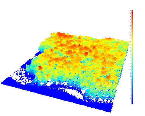
Please note, there are various options on individual tree segmentations (e.g. based on the point cloud or canopy height model). Be aware, that based on your own data, you might need to test the approaches and the results and check visually, if the results are realistic.
For a segmentation based on CHM, first the CHM needs to be generated:
# create CHM raster from point cloud with 0.5 m resolution
#(adjust values if needed)
chm_p2r_05 <- rasterize_canopy(las, 0.5, p2r(subcircle = 0.2), pkg = "terra")

# Post-processing median filter
kernel <- matrix(1,3,3)
chm_p2r_05_smoothed <- terra::focal(chm_p2r_05, w = kernel,
                                    fun = median, na.rm = TRUE)

#locate tree tops
ttops_chm_p2r_05_smoothed <- locate_trees(chm_p2r_05_smoothed, lmf(5))
# plot the CHM with the tree tops
col <- height.colors(50)
plot(chm_p2r_05_smoothed, main = "CHM P2R 0.5 smoothed", col = col);
plot(sf::st_geometry(ttops_chm_p2r_05_smoothed), add = T, pch =3)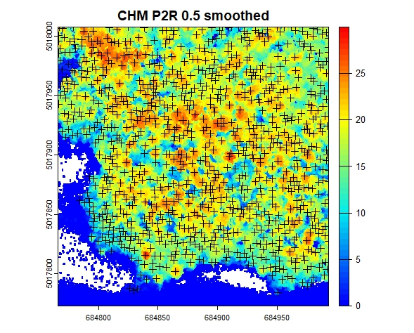
Segment the trees
algo <- dalponte2016(chm_p2r_05_smoothed, ttops_chm_p2r_05_smoothed)
las <- segment_trees(las, algo) # segment point cloud
plot(las, bg = "white", size = 4, color = "treeID") # visualize trees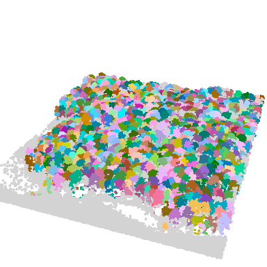
Get crown metrics
crowns <- crown_metrics(las, func = .stdtreemetrics, geom = "convex")
plot(crowns["convhull_area"], main = "Crown area (convex hull)")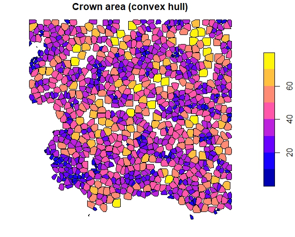
trees <- crown_metrics(las, func = .stdtreemetrics, geom = "point")
plot(trees["Z"], main = "Tree heights", pch = 16)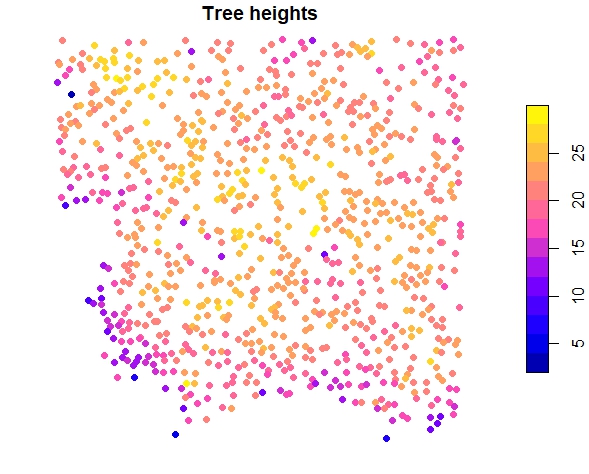
Integration into TreeCompR
Extract a inventory table from the crown data:
library(sf)
library(dplyr)
inventory <- trees %>%
  mutate(x = st_coordinates(.)[,1], y = st_coordinates(.)[,2]) %>%
  st_set_geometry(NULL)
head(inventory)
#>    treeID     Z npoints convhull_area        x       y
#> 1:     15 18.53      51        19.995 684807.0 5018005
#> 2:     16 20.66      88        39.888 684838.7 5018006
#> 3:     17 17.82      73        27.695 684892.5 5018007
#> 4:     18 13.55      51        23.316 684909.6 5018006
#> 5:     19 22.00      69        34.506 684770.2 5018006
#> 6:     20 17.75      28        19.758 684980.1 5018005
validate the inventory table with read_inv() and define
target trees (automatically) with define_targets() where
trees at the edge of the plot or dataset (1 search radius away from plot
edge) are automatically excluded for calculating CIs.
inv_trees <- read_inv(inventory, height = Z, height_unit = "m")
#> The following columns were used to create the inventory dataset:
#> id   --- treeID
#> x    --- x
#> y    --- y
#> height   --- Z
targets_buff <- define_target(inv_trees, target_source = "buff_edge", radius = 10)
plot_target(targets_buff)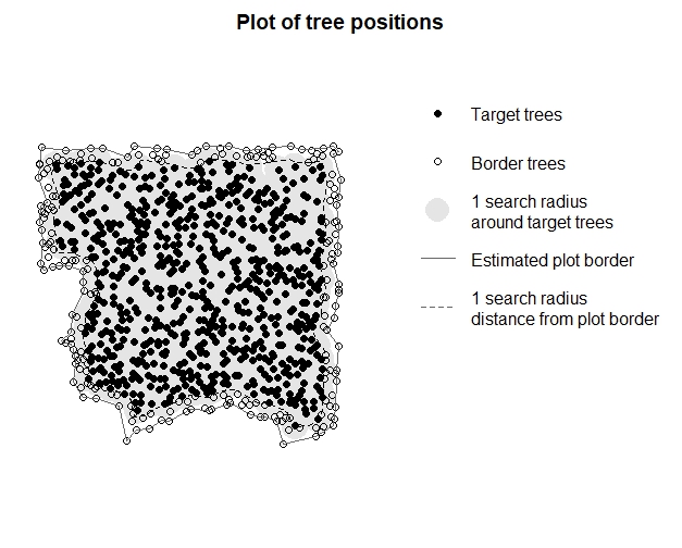
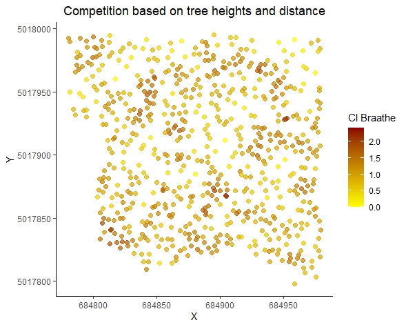
Now you can calculate the tree competition (size-distance-dependent) for your trees. Afterwards you can print your results, save the dataframe or plot the results according to your needs.
CI <- compete_inv(inv_source = inv_trees, target_source = "buff_edge",
                  radius = 10, method = "all_methods")
CI
#> ---------------------------------------------------------------------
#> 'compete_inv' class inventory with distance-based competition indices
#> Collection of data for 671 target and 220 edge trees.
#> Source of target trees: buffer around edge    Search radius: 10
#> ---------------------------------------------------------------------
#>      id         x          y height CI_Braathe CI_RK3 CI_RK4
#> 45   61 684895.13 5017995.17  17.44      0.621  3.564   5.29
#> 50   67 684812.86 5017994.96  24.26      0.494  2.633  4.222
#> 57   74 684806.23 5017990.75  25.68      1.179  7.868 10.898
#>     ...       ...        ...    ...        ...    ...    ...
#> 871 900 684966.93 5017806.91  18.44      0.737  4.914  5.585
#> 874 903 684975.75 5017803.27     19      0.705  1.173  5.863
#> 881 910 684959.15 5017797.96  16.03       0.77  3.689  5.311
plot the results
library(ggplot2)
ggplot(CI, aes(x = x, y = y, color = CI_Braathe)) +
  geom_point(size = 2, alpha = 0.7) + # Adjust point size and transparency
  scale_color_gradient(low = "yellow", high = "darkred",
                       name = "CI Braathe") + # Customizing color scale
  theme_classic() + # Change the theme
  labs(title = "Competition based on tree heights and distance",
       x = "X", y = "Y") + # Add title and axis labels
  theme(
    plot.title = element_text(hjust = 0.5), # Center the plot title
    legend.position = "right" # Position of the legend
  )
Use other size parameters to compute competition
Besides the tree height there was also the crown projection area
(“convhull_area”) of each tree as output from the ALS workflow. This
size can also be used to quantify competition, e.g. with
CI_size, a generic size-based Hegyi-type competition
index with a user-specified size-related variable
(:
size for neighbor tree
,
:
size of the target tree):
To use the crown projection area, just specify the parameter
size and the method “CI_size”:
# if the inventory data is read in outside of compete_inv() with read_inv(),
# the size column needs to be specified already in read_inv() !
inv_trees <- read_inv(inventory, height = Z, height_unit = "m",
                      size = convhull_area, keep_rest = TRUE)
CI_size <- compete_inv(inv_source = inv_trees, target_source = "buff_edge",
                  radius = 10, method = "CI_size", size = convhull_area)
#> 19 trees outside the competitive zone around the target trees were removed.
#> 872 trees remain.
CI_size
#> ------------------------------------------------------------
#> 'compete_inv' class distance-based competition index dataset
#> No. of target trees: 671    Source inventory size: 872 trees
#> Target source: 'buff_edge' (10 m)        Search radius: 10 m
#> ------------------------------------------------------------
#>       id        x       y height   size CI_size npoints
#>   1:  61 684895.1 5017995  17.44 34.948   0.618      88
#>   2:  67 684812.9 5017995  24.26 34.349   0.600      67
#>   3:  74 684806.2 5017991  25.68 34.424   1.322      69
#>  ---
#> 669: 900 684966.9 5017807  18.44 55.249   0.384      76
#> 670: 903 684975.8 5017803  19.00 53.822   0.696      75
#> 671: 910 684959.2 5017798  16.03 32.731   1.019      62

# Alternative: instead of two steps, the same can be done in one step
CI_size <- compete_inv(inv_source = inventory, target_source = "buff_edge",
                   radius = 10, method = "CI_size", size = "convhull_area")
CI_size
#> ------------------------------------------------------------
#> 'compete_inv' class distance-based competition index dataset
#> No. of target trees: 671    Source inventory size: 872 trees
#> Target source: 'buff_edge' (10 m)        Search radius: 10 m
#> ------------------------------------------------------------
#>       id        x       y height   size CI_size npoints
#>   1:  61 684895.1 5017995  17.44 34.948   0.618      88
#>   2:  67 684812.9 5017995  24.26 34.349   0.600      67
#>   3:  74 684806.2 5017991  25.68 34.424   1.322      69
#>  ---
#> 669: 900 684966.9 5017807  18.44 55.249   0.384      76
#> 670: 903 684975.8 5017803  19.00 53.822   0.696      75
#> 671: 910 684959.2 5017798  16.03 32.731   1.019      62
Other options to pre-process the ALS point clouds
There are other packages available, e.g. the itcSegment
package. Within their function itcLiDARallo(), trees are
being segmented based on typical allometric relations that can be
defined beforehand. We also used this approach with the settings below
to pre-process the MLS data in our manuscript “TreeCompR: Tree
competition indices for inventory data and 3D point clouds”. We used
publicly available laser scanning datasets from the Bavarian
Agency for Digitisation, High-Speed Internet and Surveying. For the
example below we show it with the lidR example data from above.
library(itcSegment)


# create a lookup table with common height-crown diameter-relations
# (example from itcSegment, also used in our case study)
lut <- data.frame(
  H = c(2, 10, 15, 20, 25, 30),
  CD = c(0.5, 1, 2, 3, 4, 5))

#create a digital terrain model
dtm <- grid_terrain(las = las, res = 0.5, algorithm = knnidw(k=10L, p=2))
plot(dtm)
#normalize the height of the las data by terrain
nlas <- las - dtm

# segment the trees (adjust epsg according to your coordinate reference system)
se<-itcLiDARallo(nlas$X,nlas$Y,nlas$Z,epsg=32632,lut=lut)
summary(se)
#>        X                Y              Height_m         CA_m2
#>  Min.   :684767   Min.   :5017787   Min.   : 2.51   Min.   : 0.020
#>  1st Qu.:684832   1st Qu.:5017859   1st Qu.:18.21   1st Qu.: 3.240
#>  Median :684888   Median :5017916   Median :20.52   Median : 6.120
#>  Mean   :684886   Mean   :5017910   Mean   :20.15   Mean   : 9.092
#>  3rd Qu.:684940   3rd Qu.:5017961   3rd Qu.:22.44   3rd Qu.:11.740
#>  Max.   :684993   Max.   :5018006   Max.   :29.97   Max.   :75.260
plot(se,axes=T)
# convert the SpatVector class object to a data table
inventory <- as.data.table(se)
#validate the output in TreeCompR
inv_trees <- read_inv(inventory, height = Height_m, height_unit = "m")
#>  The following columns were used to create the inventory dataset:
#>  id  --- automatically generated
#>  x   --- X
#>  y   --- Y
#>  height  --- Height_m

#quantify tree competition (adjust radius)
compete_inv(inv_source = inv_trees, target_source = "buff_edge",
            radius = 13.5, method = "all_methods")
#>  4 trees outside the competitive zone around the target trees were removed.
#>  2661 trees remain.
#>  ------------------------------------------------------------
#>  'compete_inv' class distance-based competition index dataset
#>  No. of target trees: 1973  Source inventory size: 2661 trees
#>  Target source: 'buff_edge' (13.5 m)    Search radius: 13.5 m
#>  ------------------------------------------------------------
#>          id        x       y height CI_Braathe CI_RK3 CI_RK4
#>     1:   51 684972.7 5017807  17.80      2.647 13.765 24.290
#>     2:   58 684851.0 5017807  16.37      2.718 16.880 25.298
#>     3:   59 684961.1 5017807  18.09      2.870 14.162 23.024
#>    ---
#>  1971: 2464 684849.5 5017992  12.48      7.512 45.653 75.752
#>  1972: 2468 684922.8 5017992  20.12      5.681 28.961 49.241
#>  1973: 2495 684839.2 5017992  21.96      5.172 21.985 44.906